
7.1 • Nyquist Plots 

 Frequency Response (Nyquist Diagrams)
The figure below shows the Nyquist plot for a transfer function. The poles (x) and zeros (o) of the transfer function are plotted on the complex plane. In addition the transfer function is multiplied by an adjustable gain (in green).
Use the controls to change the order of the numerator (number of zeros) and denominator (number of poles). Drag the poles and zeros on the complex plane to change their location. Complex poles or zeros are shown in the transfer function using the standard form s2 + 2ζ ωns + ωn2
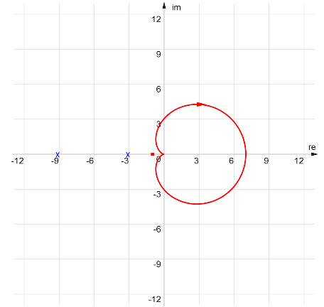 which has no encirclements of the -1 point. In additions the open-loop system has no unstable poles. Therefore:
 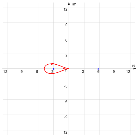 which has one encirclement of the -1 point. In additions the open-loop system has one unstable pole. Therefore:
 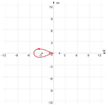 which has one encirclements of the -1 point in the counter-clockwise direction. In additions the open-loop system has no unstable poles. Therefore: