Comments...

4.0 Root Locussummarize

I n control systems it is common to design a controller with proportional gain feedback where the closed-loop system has the form

Fig 4.1 Closed‑Loop System with Unity Feedback

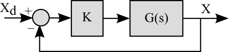
The design problem is to choose a value for k so that the closed-loop system satisfies some design specifications (see Section 2.3). The closed loop transfer function for Fig 4.1 is

X(s) _________ X_d(s)

k G(s) _________ 1+k G(s)

4.1.1

writing, G(s), as the ratio of two polynomial

G(s) =

n(s) _________ d(s)

4.1.2

and substituting into 4.1.1 we have

X(s) _________ X_d(s)

k n(s) _________ d(s)+k n(s)

4.1.3

The transient response of the system is determined by the roots of the denominator of the closed loop transfer function

d(s) + k n(s) = 0

4.1.4

The designer then needs to pick an appropriate value of k so that the roots of the polynomial (the closed-loop characteristic equation), have some desired values. The complication is that in many cases there is no value of k which results in a characteristic equation that has roots which exactly satisfy the design criteria. In these cases the solution approach is to determine all the possible roots for Eqn 4.1.4 as k is varied from 0 to ∞ and pick the k that best satisfy the design criteria.

This is the motivation for the Root Locus method. The root locus is a graph of all possible roots of a polynomial as some parameter is varied from 0 to ∞. It shows the designer every possible solution to the design problem. The designer then only need to pick a set of possible roots and find the corresponding k .

In this discussion we used a simple proportional feedback problem. However, the root locus method can be applied to most linear control system problems where the designer needs to pick a value for a single parameter.

4.1 Root Locus Construction

Given a polynomial of the form

d(s) + k n(s) = 0

4.1.5

where the parameter k is varied from 0 to ∞
where d(s) is a p^th order polynomial in s (caveat)
where n(s) is a q^th order polynomial in s
and where p >= q. (order of d(s) is larger than order of n(s))

In the previous section we provided motivation for the root locus and saw that the polynomial of interest had the form

d(s) + k n(s) = 0

where n(s) and d(s) happened to be the numerator and denominator of the open-loop system. In this section we continue using the variables n(s) and d(s) as generic polynomials even though they may not correspond to the polynomials of a transfer function.

The polynomial, Eqn 4.1.5, has p roots. We can plot a root locus (the locus of all possible roots) for 0<k<∞ by varying k, calculating the roots of the resulting polynomial for each value of k and plotting the roots on the complex plane. This is the brute force method for creating a root locus.

Fig 4.2 shows the roots of a polynomial as k is varied. Adjust the values of k to see how the roots of the equation vary with k.

s²+4 s + 3 +

(s+4) = 0 s=-3, -1

Fig 4.1 Root of a polynomial d(s) + k n(s) = 0 for various k values

Question

In Fig 4.1 what is d(s) and n(s) (answer)

d(s) = x²+4 s + 3
n(s)= s + 4
Given the equation s³ + (4 k+7)s² + (2 k+9)s + 6 = 0 what is d(s) and n(s) (answer)
Rewrite the equation by separating terms multiplied by k from those not multiplied by k. This gives:
d(s) = s³ + 7 s²+9 s + 6
n(s)= 4 s² + 2 s

Root Locus Approximations

In many design cases we don’t need an exact root locus. We instead need a approximate root locus so we can determine if the proposed controller configuration is capable of achieving the performance specification. There are several rules that help us approximate a root locus. On this site we present a simple set of rules. See a controls text for a complete set.

Rule 1

The root locus has p points associated with every k. This follows because Eqn 4.1.5 is an p^th order polynomial and so must have p roots. (help)

d(s) is a polynomial of order p
n(s) is a polynomial of order q
where p ≥ q

Rule 2

The root locus is symmetrical about the real axis. This follows because all of the complex roots of Eqn 4.1.5 must be complex conjugate pairs.

Rule 3

When k=0 the roots of the Eqn 4.1.5 are the roots of d(s)=0 - this rule should be obvious.

Rule 4

When k = ∞ the roots of Eqn 4.1.5 are the roots of n(s)=0. This rule make sense as long as the order of n(s)=0 is the same as the order of d(s)=0. In this case the polynomial k n(s)=0 dominates Eqn 4.1.5 because k is very large and so the roots of the equation are the roots of n(s)=0. However, if the order of n(s) is less than that of d(s) we are missing (p-q) roots (see Rule 1). In that case we use Rule 5.

Rule 5

When the order of n(s) is less that the order of d(s) there are (p-q) roots at infinity when k = ∞. See a control text for the mathematical details (convince me by example). The location of these roots at infinity follow a specific pattern depending on (p-q). That pattern is shown in Fig. 4.3. In the figure, the patterns are centered on the origin. However, the pattern center varies and dependes on the poles and zeros of the system. The center of the pattern on the real axis, x, is

x =

∑ (poles) - ∑ (zeros) _________ p-q

For the equation

s+k=0

d(s)=s and n(s)=1. Hence p-q=1 so there should be 1 zero at infinity. Set k=∞ then

s + ∞ = 0

which has a root at s = -∞

For the equation

s² + k=0

d(s) = s² = 0 and n(s)=1. Hence p-q=2 so there should be 2 roots at infinity. Set k=∞ then

s²+∞=0

which has roots at s = ±∞ i

( p - q ) = Order of d(s) - Order of n(s) =

Fig 4.1.1 Location of roots when p-q >0

4.2 Root Locus for Unity Feedback

Root locus can be used to analyze the characteristic equation of any system. However, when the system uses proportional gain with unity feedback the technique has a simple interpretation (this was discussed at the beginning of this chapter, but its repeated here for clarity).

Given a closed loop system with proportional feedback

Fig 4.1 Closed Loop System with Unity Feedback

where

G(s) =

n(s) _________ d(s)

the closed-loop characteristic equation is

d(s) + k n(s) = 0

This has the same form as Eqn 4.1.5. Notice that the poles of G(s) are the roots of d(s) = 0 and the zeros of G(s) are the roots of n(s) = 0. In control systems design we say that theThe root locus of G(s) starts at the poles of G(s) and ends at the zeros of G(s).

Remember this is a special case where the system has the form of Fig 4.1. If the system does not have this form, find the closed-loop characteristic equation and use algebra to put it in a form d(s)+ k n(s) = 0 where d(s) and n(s) are some polynomial, not necessarily the numerator and denominator of G(s).

Root Locus Experiment

Use the following experiment to build some intuition about the root locus for different systems. Notice that the root locus pattern is related to the relative position of the roots of d(s) = 0 and n(s) = 0

Root Locus

Exercise

Sketch the approximate root locus for the following polynomial. Then use the root locus tool to verify your results.

s³+k s² + 16s + 4k = 0

Hint: (show)

Rearrange the polynomial into the form d(s) + k n(s) = 0

s³+ 16s + k (s² + 4) = 0

Therefore d(s) = s³+ 16s, which yields poles at s = 0, +4i, 14i and n(s) = s²+ 4, which yields zeros at x= +2i, -2i

The root locus has three branches, which start at 0, +4i, -4i. The branches end at the zeros +2i, -2i and -∞ on the real axis.

Homework

Links to relevant homework:

Links go here