Comments...

5.0 Frequency Analysis

T he root locus approach discussed in previous chapters is a technique for analyzing differential equation and designing control systems in the time domain. An alternate approach is to do the design in the frequency domain. In the time domain we used Laplace transforms. In the frequency domain we will use Fourier transforms. Fortunately, Laplace and Fourier and transforms are closely related (remind me).

Frequency domain analysis is useful because it provides a different perspective on control systems design - and sometimes a different perspective makes the design process easier or gives some insight. In some cases its also possible to generate the frequency domain model experimentally, eliminating the need to develop an analytical model.

5.1 Bode Plots

A Bode plot is a plot of the frequency response of the system at steady state. The frequency response of a system can be found by exciting the input with a sinusoidal frequency with an amplitude of one. Differential equations theory tells us that the output of the system will also will be sinusoidal with the same frequency as the input sinusoid but may have a different magnitude and phase.

Figure 5.1 show the input and output for a simple transfer function. Vary the input frequency and observe how the output changes in both the amplitude and the phase.

The Bode plot is a graph showing the magnitude and phase of the output as a function of frequency. Frequency is measured on a log scale. Magnitude is measured in decibels (remind me) The figure below shows the Bode plot (frequency plot) for the system in Fig 5.1. The green line indicate the current frequency selected in that figure.

Questions

1. How does the input and output amplitude compare for low frequencies (around 2r/s) (answer).
   At low frequencies the input and output have the same amplitude. This is expected. Verify that the steady-state gain for the system is 1 by using the final value theorem

   limt → ∞ f(t) = lims → 0 s F(s)

   and using a step input (1/s)
2. How does the input and output amplitude compare for frequencies greater than 20 r/s (answer).
   At high frequencies the output is attenuated. The transfer function is a low pass system so we expect that it will attenuate high frequency signals
3. What happens to the system gain at 10r/s (answer).
   From the standard form

   s² + 2 ζ ω_n s + ω_n²

   the systems is under damped with a natural frequency of 10r/s. When in input is 10r/s it excites the natural frequency and amplifies the input.
4. How does the phase of the output signal differ from that of the input?(answer).
   The input and output are in phase for low frequencies. Around 8r/s there is a noticeable phase shift in the output. Above 12r/s the output is 180° out of phase with the input.

Bode Plots - Brute Force

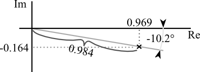
Given a transfer function you can compute the magnitude and phase shift at a given frequency by making the substitution, s = j ω. The magnitude is the magnitude of the resulting complex value, and the phase is the phase angle of that value.

For example, compute the frequency response for (math help)

Given the complex number

10(5) j____________(j5)²+50j + 16

=

50 j____________-9 + 50 j

multiply the numerator and denominator by the complex conjugate of the denominator and simplify

50j____________-9 + 50 j

-9 - 50 j____________-9 - 50 j

=

2500 -450 j____________9² + 50²

= 0.969 - 0.174 j

Plot the value on the complex plane and compute the magnitude (0.984 or 20log(0.984)db = -0.14db) and phase (-10.2°)

To create a Bode plot, calculate the gain and phase for 0 < ω < ∞ and plot the values. This of course, is not very practical with out the use of a computer. However, you can quickly sketch a Bode plot using linear approximations.

Bode Plots - Approximations

The brute force method described above always works, but is not practical without a computer. In most cases an approximation is adequate and can be drawn using a few simple rules.

To create an approximation of the Bode plot, start by separating the transfer function into the product of real poles and zeros, and complex poles and zeros. Then sketch the approximation for each pole and zero then graphically add all of the plots together. This works because Bode plots are drawn on a log scale. To multiply factor you add them in log space. (trivia) The following figures show the approximations for different pole and zeros combinations (Single sheet view) Notice that for each case we have divided out the gain so that the DC gain is unity (explain)

A slide rule was used before the advent of calculators. You could multiple numbers together by moving two log-scales with respect to each other. Adding the distance on the log scale graphically results in multiplying two values together. Wiki page on slide rules

G(s)= K A constant has the same gain at all frequencies. On the bode plot this is a straight line at 20log(K). The phase shift is zero for all frequencies. G(s) = 1____________s The frequency response of an integrator has a infinite gain 0 frequency (10-∞;), a gain of zero at an infinite frequency (10+∞;)and a gain of 1 (0db) at 1 rad/sec. The phase shift for an integrator is -90° G(s) = s The frequency response of an derivative has a gain of 0 at 0 frequency (10-∞;), an infinite gain at an infinite frequency (10+∞;)and a gain of 1 (0db) at 1 rad/sec. The phase shift for an integrator is +90° Notice the similarities and differences between a differentiator (s) and integrator (1/s) G(s) = 1____________s/a+1 A pole at s = -a has a constant gain up until a rad/sec, then the gain decreases at a rate of -20db/decade (where a decade is 10x rad/sec). a rad/sec is called the "break point". The pole has a total phase shift of -90°. The phase is 0 at 0.1a rad/sec, -45° at a rad/sec; and -90° at 10a rad/sec. Notice the transfer function is written so that the constant gain of the system is 1 (limit s → 0). G(s) = s/a+1____________1 A zero at s = -a has a constant gain up until a rad/sec, then the gain increases at a rate of +20db/decade (where a decade is 10x rad/sec). a rad/sec is called the "break point". The zero has a total phase shift of +90°. The phase is 0 at 0.1a rad/sec, +45° at a rad/sec; and -90° at 10a rad/sec. Notice the transfer function is written so that the constant gain of the system is 1 (limit s → 0). G(s) = 1____________s2/ωn2 + 2ζ/ωn + 1 A complex pole with a natural frequency of ωnhas a constant gain up until approximately ωn rad/sec, then the gain decreases at a rate of -400db/decade (where a decade is 10x rad/sec). a rad/sec is called the "break point". The poles have a total phase shift of -180°. The phase is 0 at 0.1ωn rad/sec, -90° at ωn rad/sec; and -90° at 10ωn rad/sec. Notice the transfer function is written so that the constant gain of the system is 1 (limit s → 0). G(s) = s2/ωn2 + 2ζ/ωn + 1____________1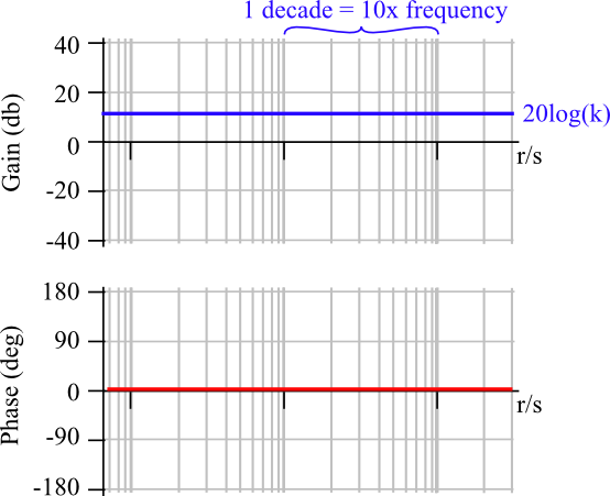

Bode Plot Example 0:00

Bode Plot Experiment

Bode Plots